This tutorial walks through the basic steps required to create a simple task graph, configure network topology, and evaluate the end result in a simulator. It shows how the tool automatically maps user-defined task graph to a set of suitable network nodes.
Table of Contents
Starting up
Follow the installation instructions.
After downloading and building the software, go to the top directory and execute the command ./run.sh
Then open browser at http://localhost:12000/profun.
Task graph
In order to create a taskgraph, click on a node in the palette tab (left side) and drag it on the main working area.
This simple example creates an application that consists of two communicating tasks. We use inject node to input some values in the network and print node to print these values.
Drag inject task from palette, then drag the print task. Link the tasks together to get the following layout:
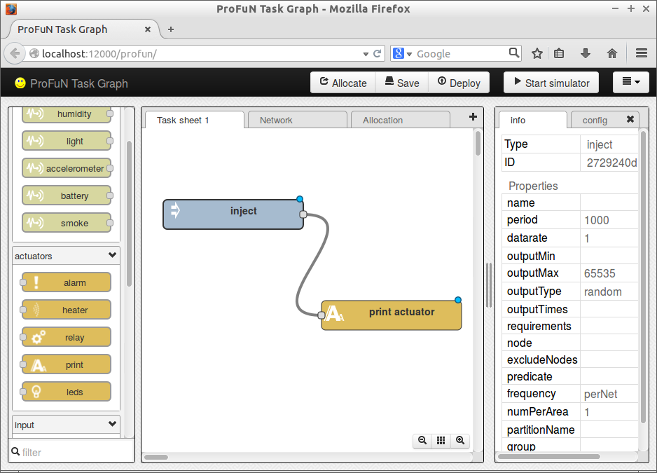
A task is a basically a software compoent. Some tasks also correspond to some hardware components (actuators, sensors), but many do not, such as data processing or controller tasks.
A task has a number of configurable properties, zero or more inputs, and zero or more outputs. Inputs are always shown as small rectangles on the left side of a task, outputs on the right side.
For the print task, not much configuration is required. inject task, on the other hand, can be configured by specifying the range of the values it will output, and the ordering of values in this range (random / increasing / decreasing).
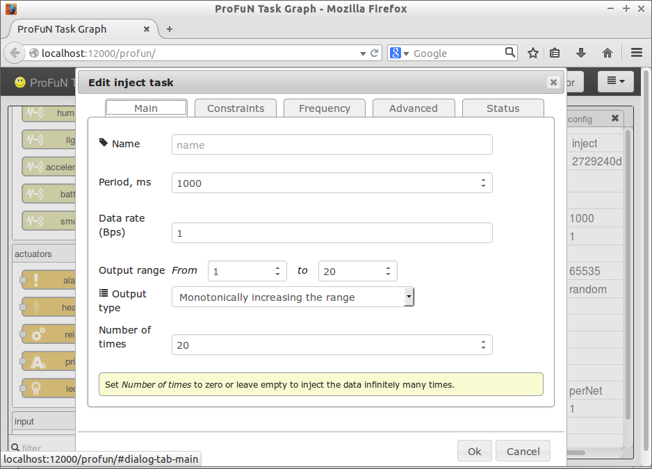
Open the configuration dialog by double clicking on the inject task.
For a test, let’s make it print numbers from 1 to 20 in increasing order, and then stop. To do that:
-
Change “Output range”, set “From” equal to 1 and “To” equal to 20.
-
Change “Output type” to “Monotonically increasing”.
-
Change “Number of times” to 20.
Press OK. The changed properties are now displayed in the inject task rectangle:
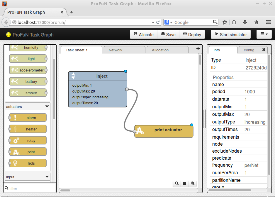
Congratulations! The application is ready to be tested.
Network
Switch to network tab. Initially it’s empty, so drag some nodes from the palette to populate it. We will be using Zolertia Z1 nodes throughout this tutorial.
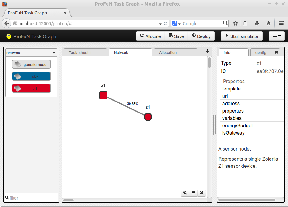
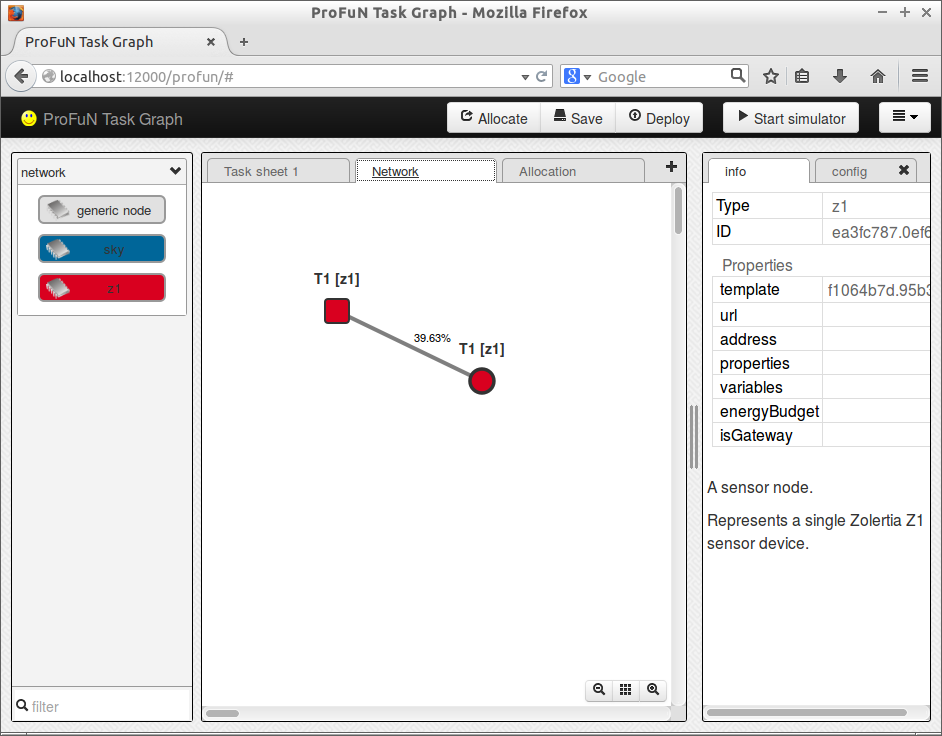
Gateway / base station nodes are displayed as rectangles, other nodes are displayed as circles.
- Tip: by default, the “big” rectangles with property lists are not displayed it the network tab. To change this, go to “Visual options” dialog and mark the checkbox.
The links between the nodes are automatically added by the network simulator running in background if it detects that the nodes are within the configured radio-reachability radius.
On top of the link between the nodes, link’s quality estimate is printed. In this case, its just 39.63%. That means that less than 40% of all packets transmitted from one endpoint of a link will reach the other endpoint.
- Tip: You can manually change the link quality values by double-clicking on the link and editing its configuration.
Each node can be configured to have a distinct list of hardware components (sensors, actuators) and capabilities. However, in a typical sensor network, many nodes are going to share hardware capabilities. It would be a bad idea to require to specify the list for each node individually. Instead, the list can be specified once, in the template of a node. Then this template can be reused for other nodes.
Nodes created by copying an existing node and pasting (Ctrl+C, Ctrl+V) the result are going to inherit the template from their originals. However, nodes created by dragging do not have a preconfigured template, and are therefore by default invalid. No tasks can be mapped to these nodes.
To fix this problem, double-click on a node to open its configuration dialog. The border around the field “Template” is red, which means that the value in the field is invalid. Click on the small button at the right side:
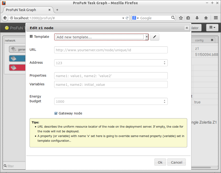
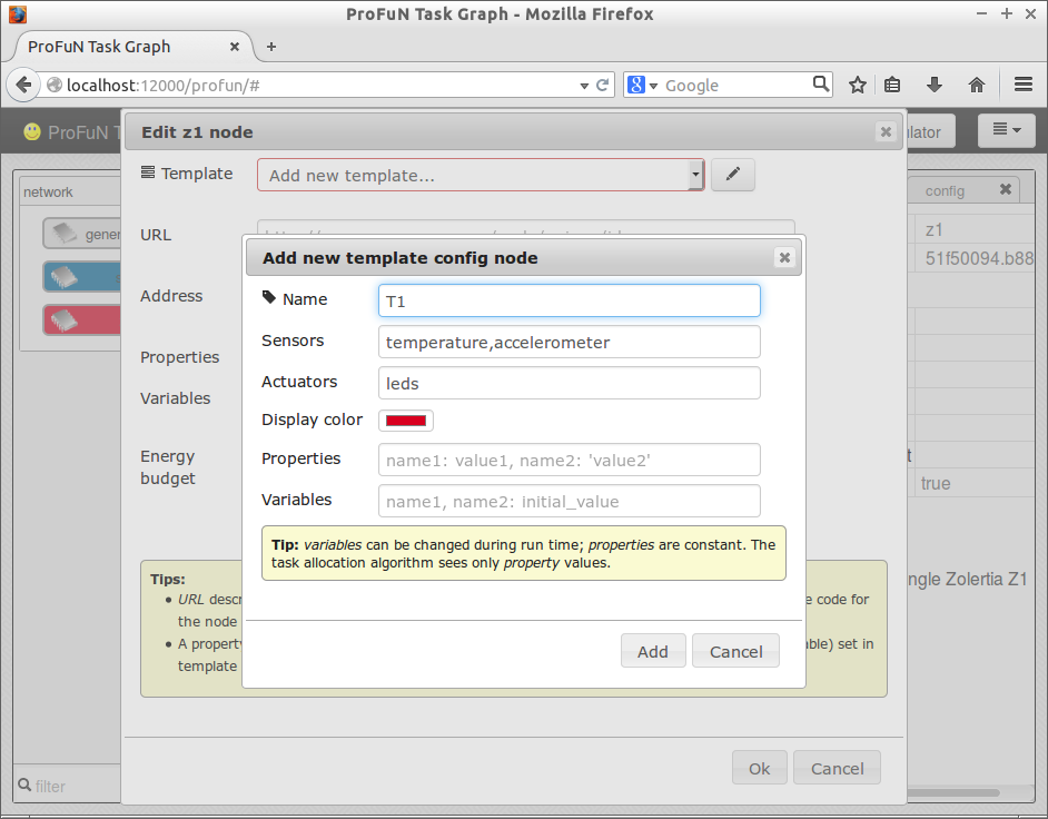
The template already suggests which sensors and actuators are on-board for this type of node (Zolertia Z1). You can add or remove them, but for now just enter your own name for the template and click “Add”.
Confirm the template by exiting the node configuration dialog with “Ok”. Also, configure (select and confirm) the same template for the other node:
Allocation
You might want to save your work before continuing. To do that, press the “Save” button. Now the model that you have designed is stored in permanent memory. (In Node-RED terminology, models are called flows. However, here the model it includes not only the task graph itself, but also the network and all kinds of options. Models are stored on disk and exchanged between different components in JSON syntax.)
The saved model is typically stored on the server, unless you have read-oly access to the server - in that case the modified model is stored locally, in web browser’s persistent storage. The model that was saved last can be recalled by simply refreshing the page; that causes all unsaved state to be lost.
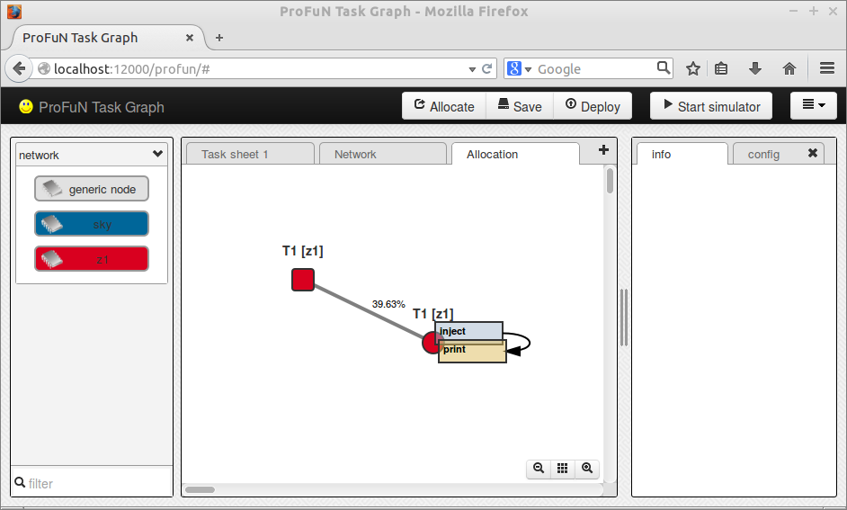
Now press the “Allocate” button. Several things should happen.
First, the model is sent to the task allocator daemon. The daemon figures out the most energy-efficient way in which tasks can be mapped to the network, while still satisfying all their constraints, such as hardware requirements. (At least by default the tool optimizes for energy efficiency; other so-called objective functions are possible that may optimize for other metrics). In our scenario, that means the communicating task pair will always be put in the same node, as the tasks do not have any specific requirements for hardware components.
The daemon replies with the resulting mapping, which is a simple JSON message. You can look at the window where the task allocator is running to see it:
{"mapping": [{"taskId" : 0,
  "mappedOnNodes" : [
  {   "nodeId" : 1,
      "destinations" : [{ "node" : 1, "task" : 1 }]
  }]
},
{"taskId" : 1,
  "mappedOnNodes" : [
  {   "nodeId" : 1,
      "destinations" : []
  }]
}]}
The result is displayed by the frontend:
Seeing it in action
The model that you have designed can be tested using a network simulator. There should be a simulator running in a separate window with a title “ProFuN empty template” if you’ve started the tool with ./run.sh script.
When you now press the “Start simulator” button, the first thing that the simulator does is to create firmware images for all the network nodes. This usually takes some time (20-30 seconds), and the firmware includes both Contiki operating system and ProFuN-specific layer of middleware. The middleware takes care of taskgraph’s runtime management; the firmware for a node also includes hardware component drivers, definitions of properties configured in its template, and definitions of properties configured in nodes own configuration dialog. The nodes that have an identical set of components and properties use an identical firmware image.
After the build is finished, the simulator should start executing the firmware images. You can pause the simulator any time by pressing the “Pause simulator” button. Further restarts of the taskgraph won’t require recompilation, unless you modify configuration of network nodes (components or properties).
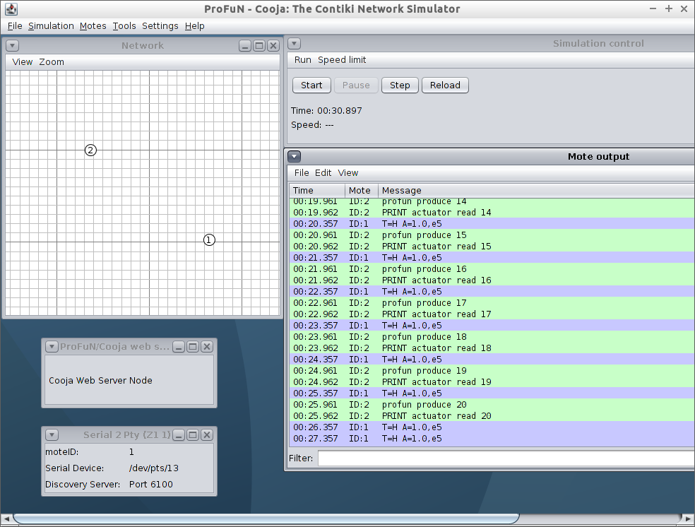
Switch to the simulator window. The “Mote output” sub-window should show that:
-
Contiki has started on both nodes;
-
task setup messages are received by the gateway node and forwarded to the other node;
-
tasks are started on the other node;
-
the inject task is periodically producing data, and the print task is periodically printing data, until all numbers from 1 to 20 are printed (and then stopping).
The end result should look like this:
If something goes wrong (e.g. the simulator is running, but tasks are not started), check the console tab where the gateway daemon is running, or its log file. The daemon, among other tasks, prints task mapping status information. To set up tasks, ProFuN frontend does not set communicate with the simulator directly; instead, it sends the model to a gateway daemon, which in turn talks with the simulated gateway node using a virtual serial port. This approach has the benefit of working both with simulator and with real sensor nodes.
Download
The resulting model file is available here.